Background

Consumers at the domestic and industrial level are frequently confronted with the need to select steel products that are already galvanised. The fact that they are ‘galvanised’ is used as a major selling point. In many cases, the standard of the ‘galvanised’ coating may not be not clearly represented, and in some cases, misrepresented.

Claims may be made by the manufacturer that are not able to be substantiated in the field. With other products, particularly those that are zinc plated, descriptions such as ‘galvanised’ are used on the packaging that deliberately mislead buyers into expectations of durability that will never be realised.

More and more products are being introduced that are galvanised by high-speed, in line galvanizing technology. This allows a thin zinc coating to be applied to the steel at low cost. These thin zinc coatings are frequently coated with clear polymer topcoats to enhance their storage characteristics and in some cases, claims have been made that the addition of these polymer topcoats significantly improves the durability of the coating compared to a conventional galvanised coating. The addition of organic coatings to zinc plated parts is also a common technique that the manufacturers claim improves the corrosion resistance of their products. What are the facts?

Coating Characteristics

Zinc Plating

Zinc plating involves the electrolytic application of zinc by immersing clean steel parts in a zinc salt solution and applying an electric current. This process applies a layer of pure zinc that ranges from a few microns on cheap hardware components to 15 microns or more on good quality fasteners. Technical and cost issues prevent the economical plating of components with heavier coatings.

In-Line Galvanised Coatings

In-line galvanised coatings are applied during the manufacturing process of the hollow or open section, with the cleaned steel section exiting the mill and passing into the galvanizing bath. This process applies a coating of zinc to the surface that can be controlled in thickness. This coating is usually measured as coating mass in grams per square metre and ranges from a minimum of about 100 g/m² upwards, with an average around 175 g/m².

Accelerated Weathering Testing

Accelerated weathering testing of coatings has traditionally been done in salt spray cabinets. This testing technique has been largely discredited with respect to metallic coatings as it does not reflect the way metallic coatings weather in atmospheric exposure conditions where the development of stable oxide films gives these coatings there excellent anti-corrosion performance. The addition of polymer topcoats to metallic coatings will significantly improve their apparent performance in salt spray tests but field performance will not necessarily reflect this.

Finding the Facts

The South African Bureau of Standards has recently undertaken accelerated weathering trials of polymer coated in-line galvanised coatings and compared them with conventional in-line galvanised and hot dip galvanised coatings to evaluate the effect on durability of the addition of these this polymer topcoats. A summary of this report follows.

S.A.B.S. Report

The samples were subjected to Salt Fog testing, Damp SO₂ Atmosphere testing and QUV Weatherometer testing as well as Hardness testing. The conclusion of the SABS report states the following;

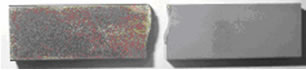
"The results of the accelerated corrosion tests indicate that the expected life of the continuously galvanised and lacquer coated samples will not be essentially different from the commercially continuously galvanised sheet material. Test results demonstrate that the expected life exhibited by the standard hot-dip galvanised panels (zinc coating thickness approx. 100 microns) can be considered to be significantly superior to the continuous galvanised/lacquer samples. The lacquer coating appears not to be fully effective in inhibiting the onset of corrosion under damp conditions due to porosity.

It is well known that the zinc/iron alloy layers of standard hot-dip galvanised coatings are hard in nature (in excess of 200HV - often harder than the base steel itself). Conventional hot-dip galvanised coatings, consisting of alloy layers with a soft zinc outer layer, therefore provide in essence a buffer stop coating which withstands knocks and abrasion. The soft nature of continuous galvanised lacquer coating (75 HV) coupled with the low coating thickness indicates that these coatings will not have the same ability to withstand rough handling compared to conventional hot-dip galvanised items."

Poor Performance from Plated Coatings

Zinc plated coatings are not suitable for exterior exposure applications. Zinc plated bolts and hardware fittings such as gate hinges will not provide adequate protection from corrosion, and will rarely last more than 12 months in exterior exposures in most urban coastal environments.

Zinc plating has been used in industrial coating applications from time to time, with very poor results. Industrial Galvanizers joint venture galvanizing operations in Bakasi, Indonesia, PT Bukit Terang Paksi Galvanizing (BTG), was commissioned in March 1998 to reprocess a large tonnage (approx. 400 tonnes) of cable trays that had been electroplated. The zinc electroplated coating had failed prior to delivery to the project resulting in the rejection of the entire consignment.

The client requested an extra-heavy hot-dip galvanised coating to replace the zinc plating, and BTG was able to apply a 100 micron coating to the 3 mm thick cable tray sections - this is around 50% above the required minimum standard for hot dip galvanised coatings applied to steel of this thickness of and over 10 times the thickness of the zinc plating.

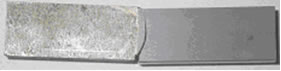
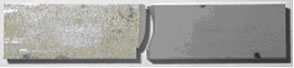
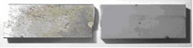
Zinc plated products have an attractive appearance when new as the zinc coating is bright and smooth, where a hot dip galvanised coating has a duller and less smooth surface. There is typically about 10 times as much zinc applied to small parts in the hot dip galvanizing process as with zinc plating. A bright, shiny smooth zinc finish on builders hardware (bolts, nuts, hinges, gate latches, post shoes) indicates a plated coating that will not provide adequate corrosion resistance and will rarely provide more than 12 months protection in most of the coastal population centres.

Background

There are many instances where hot dip galvanised coatings need to be painted. There are well established quality assurance procedures for the painting of hot dip galvanised components in a controlled environment, but it is a common requirement to apply paint coatings to hot dip galvanising on site.
Surface Condition

When a steel item is first hot dip galvanised, its surface is free from oxidation and contamination and is in the best condition for coating and is also highly susceptible to oxidation, particularly reaction with atmospheric moisture. Most galvanisers quench the work in a weak sodium dichromate solution to passivate the surface. This chromate passivation film weathers away with time and is replaced by a stable complex carbonate oxide film. This dynamic set of surface conditions needs to be considered when painting galvanised steel.

In addition, surface contamination can occur that will interfere with paint adhesion. Diesel fumes are a common source of surface contamination that are very difficult to detect, as the galvanised coating may still appear clean and bright.

Where close control of surface condition is not possible, the best alternative to ensure a high quality paint application is to brush or sweep blast the galvanised surface immediately prior to painting. This is a poorly understood technique with many paint contractors. Incorrect technique will cause serious damage to the hot dip galvanised coating.
Abrasive Blasting

The following specification is recommended for abrasive blasting of hot dip galvanised surfaces prior to painting. Compliance with this specification will ensure that not more than 10 microns of zinc will be removed from the galvanised coating during the blasting process, and that the coating will not be damaged by fracturing of the alloy layers through excessive impact energy of the blast media on the galvanised coating.
Brush or Sweep Blasting Procedures for Preparing Hot Dip Galvanising for Painting

1. Blast nozzle pressure 50 psi (350 kPa) maximum

2. Abrasive grade 0-2 - 0.5 mm

3. Abrasive type - clean ilmenite or garnet

4. Distance of nozzle from surface 400 - 500mm

5. Nozzle type - 12mm minimum diameter venturi type

6. Blasting angle to surface - 45 degrees

The aim of this blasting procedure is to remove any oxide films and surface contaminants from the surface. It is not to produce a profile similar to that required on bare steel. The brush blasting of the relatively soft zinc will automatically produce a fine profile, giving the clean surface a satin appearance.
Inexperienced Operators

With inexperienced operators, a test section should be evaluated by measuring coating thickness before and after blasting with an approved magnetic thickness gauge. A 5-10 micron reduction in galvanised coating thickness indicates an acceptable technique. Over 10 microns of coating removed indicates an unacceptable technique.
Other Surface Finishes

On reactive steel, the coating may already have a matte grey or satin appearance. This indicates the presence of the zinc-iron alloy layers at the surface, which also indicates a thicker than standard galvanised coating.

The micro-roughness of the alloy layers already provides a good mechanical key for appropriate paint, and only very light brush blasting is required on galvanised coatings of this type.

Grey galvanised coatings are more susceptible to mechanical damage than shiny coatings and should be treated accordingly.

While hot dip galvanising is usually priced in dollars per tonne, it is desirable to also convert this to dollars per square metre to allow comparison with alternative coatings.

In addition, the conversion to square metres allows accurate estimation of weight increase through the addition of the hot dip galvanised coating. The surface area per tonne can also be calculated using the following formula:

Surface Area per tonne = 255/Section Area in mm

Mass per square metre of steel can be calculated using the following formula:

Mass per Square Metre (g/m²) = Section Thickness (mm) x .85

Section Thickness (mm)	Surface Area/Tonne (m2/tonne)	Mass/m2 kg/m2	Min Coating Thickness (µm) per AS 1650*	Mass Increase (%)**
1mm	255	7.85	45µm (320g/m2)	4.10
2mm	127	15.70	55µm (390g/m2)	2.85
3mm	85	23.55	55µm (390g/m2)	1.65
4mm	64	31.40	70µm (500g/m2)	1.59
5mm	51	39.25	70µm (500g/m2)	1.25
6mm	42	47.10	70µm (500g/m2)	1.05
8mm	32	62.80	85µm (600g/m2)	0.95
10mm	25	78.50	85µm (600g/m2)	0.75
12mm	21	94.20	85µm (600g/m2)	0.65
15mm	17	117.75	85µm (600g/m2)	0.50
20mm	13	157.00	85µm (600g/m2)	0.40
25mm	10	196.25	85µm (600g/m2)	0.30

* Hot rolled steel sections and heavier steel sections will generate galvanised coatings considerably thicker than required by the AS 1650 Standard. To convert coating thickness in microns to equivalent coating mass in grams per square metre (g/m 2 ), use the following formula:

Coating mass (g/m²) = Coating Thickness (µm) x 7.05

Coating Thickness (µm) = Coating Mass (g/m²) x 0.14

** Actual zinc pickup after galvanising will depend on average coating thickness and section design.

Poor drainage, zinc entrapment and large horizontal surfaces will result in higher zinc pickup.

Note: Actual zinc usage in hot dip galvanising is significantly higher than physical zinc pickup. Zinc usage in hot dip galvanising is typically 5-7% of the mass of steel dipped because of zinc consumed on jigs and in generating zinc ash and zinc dross in the galvanising process.

Background

Galvanised coatings have an unusual characteristic compared to other protective coatings in that they fail by weathering and oxidation from the surface. Paint coatings, once breached, deteriorate through under-film corrosion and can suffer rapid failure as a result. Because of the electrochemical protection provided to steel by zinc (galvanised) coatings, no corrosion of the steel will occur while there is any zinc present, regardless of the thickness or condition of the galvanised coating. Galvanised coatings, in atmospheric exposure conditions, corrode at an approximately linear rate. Once this rate has been established for a particular environment, the expected life of the coating can be defined by relating the rate of corrosion to the thickness of the coating.

Factors Affecting Galvanised Coating Life

The durability of galvanised coatings depends on a number of environmental factors. These include: · Time of wetness · Ambient temperature · pH of moisture · Chloride levels in atmosphere · Sulfate levels in atmosphere · Contact with other chemicals · Contact with dissimilar metals · Orientation of exposure (vertical, horizontal) · Nature of exposure(sheltered, open) · Ventilation conditions Corrosion engineers take these factors into account when assessing the life-cycle performance of galvanised coatings. Organisations such as the CSIRO have developed environmental assessment techniques based on atmospheric computer models that facilitate the accurate assessment of metallic corrosion rates. A number of international (ISO) standards have also been developed that use combinations of the parameters listed above to tabulate corrosion rate data for zinc (galvanizing) and other metals. Classification Of Environments Most standards and documents associated with coating performance use exposure classifications to define corrosivity of the atmosphere. For metallic coatings such as galvanizing, factors such as UV exposure do not impact on coating life, where with paint coatings, UV levels are an important factor in their durability. For galvanised coatings, common Australia exposure classifications are arid/rural, mild/urban, industrial, marine and tropical. Much exposure testing has been done to obtain corrosion rate data in these environments, and this work is ongoing. Testing done in a number of long-term case studies has indicated that hot dip galvanised coatings in service may have lower corrosion rates than those of zinc coupon samples exposed in test facilities. Reasons for this apparent lower rate of in-service corrosion have not been quantified, but are thought to be related to the quite different characteristics of a hot dip galvanised coating compared to pure zinc, typical of the samples used in exposure testing. The hot dip galvanised coating contains alloys of iron, aluminium and sometimes nickel, each of which may modify the way the coating reacts with the environment. The following table shows typical corrosion rates of hot dip galvanised coatings in the various environmental classifications. Table 1. Corrosion Rates of Hot Dip Galvanised Coatings Environment Corrosion Rate – microns/year Arid/Rural <1 Mild/Urban* 1-3 Industrial 3-5 Marine** 5-15 Tropical 1-3 * Metropolitan and urban areas within 25 km of the Australian coastline outside the ocean surf spray zone. ** Within the ocean surf spray zone from 0 – 1000 metres from ocean surf, depending on topography. Coating Thickness Versus Coating Life All continuously galvanised and after-fabrication galvanised steel products have coating thickness specified in various Australian, New Zealand and international standards. By relating this coating thickness to the corrosion rates in the table, an accurate estimate of galvanised coating life can be obtained. Hot dip galvanised coatings that comply with AS/NZS 4680 – 1999 are those that will give the longest life, as they are typically 3 –5X the thickness of zinc coatings applied to continuously galvanised products. On structural steel sections, 50 years life before first rust in other than marine or heavy industrial environments is a reasonable expectation. Case history studies of existing installations in tropical and industrial environments indicate that 100 year life is achievable with galvanised coatings applied after fabrication.

Background

Galvanic corrosion may occur when two dissimilar metals are in contact in an electrolyte (this includes most aqueous solutions).

Except for graphite, stainless steel is the noble metal in most galvanic pairs. Hence it is protected at the expense of the other metal when in contact, for example, with iron, steel, aluminium, zinc or cadmium. The solution to this problem lies in using, so far as possible, metals of the same composition for complete assemblies when this condition is encountered. In some cases an insulating lacquer or gasket can be used as a separation between two metals at the point of contact.

The following table shows the galvanic behaviour of stainless steels with other metals when tested in sea water.

Galvanic Corrosion of Metals in Sea Water

If two metals in this list are in contact with sea water, then the metal nearest the top of the list is the one most likely to corrode at the metal junction. The degree of corrosion is increased as the separation of the alloys in the list is increased. Potential differences of less than 100mV are unlikely to cause problems. However, the relative areas of the two dissimilar metals are also important - the higher the ratio of the areas of the noble metal to active metal, the greater will be the corrosion and vice versa.

Table 1. Galvanic series of metals and alloys in seawater.

Active

Magnesium

Magnesium alloys

Zinc

Aluminium

Cadmium

Steel

Cast iron

Chromium iron (active)

18-8 chromium-nickel-iron (active)

Titanium (active)

Lead

Tin

Nickel (active)

Brasses

Copper

Bronzes

Copper-nickel alloys

Silver solder

Nickel (passive)

Chromium-nickel (passive)

18-8 chromium-nickel-iron (passive)

18-8-3 chromium-nickel-molybdenum-iron (passive)

Titanium (passive)

Silver

Graphite

Zirconium

Gold

Platinum

Noble

Abstract

Fracture toughness tests were carried out for Si3N4/S45C specimens with interface cracks of different lengths. It was found that the specimen with a crack of 4 mm has higher apparent fracture toughness than those with cracks of 1 mm and 2 mm due to the reduction of the residual stress. Fracture propagated into Si3N4 from the crack tip in the direction of 40o for cracks of 1 mm and 2 mm while it propagated along the interface for crack of 4 mm. Elasto-plastic analysis was carried out considering S45C as the linear hardening material and Si3N4 as the elastic material. It was found that the stress around the crack tip is dominated by an elasto-plastic singular stress field, which is substantially the same as the elastic singular stress field of an interface crack. Evaluation of the fracture path and toughness was carried out based on the stress intensity factors of the elasto-plastic singular stress field.

Keywords

Interface Crack, Fracture Toughness, Si3N4/S45C Joint, Thermal Residual Stress, Elasto-plastic Analysis

Introduction The ceramic/metal joints have been increasingly applied in a wide range of engineering fields because the ceramic has stable mechanical properties at high temperature and good resistance to wear, erosion and oxidation. However, the difference of material properties between metal and ceramic induces stress singularities at the interface edge. Moreover, high thermal residual stress will be induced during the cooling process due to the mismatch of the thermal expansion coefficients. The stress singularity together with the thermal residual stress degrades the strength of ceramic/metal joint and makes the evaluation of the strength difficult. Many works have been done about the residual stress and the strength evaluation of ceramic/metal joints. For example, Kobayashi et al. [1, 2] have investigated the bending strength and residual stress of Si3N4/S45C joint and the effect of the size of the specimen on the bending strength. Qiu et al. [3] have investigated the influence of residual stress and cyclic load on the strength of Si3N4/S45C joint. However, due to the complexity of the problem, a generalized evaluation method for the ceramic/metal joint has not yet been proposed. The elastic solution of the singular stress field of the interface crack has been studied since 1959 [4-9]. Rice [10] has summarized the work in this field and set up the elastic fracture mechanics concepts for interfacial cracks. Yuuki et al. [11, 12] have proposed the maximum normal stress criteria for predicting fracture path and strength of ceramic/metal joint based on the elastic theory. The plastic deformation of metal will inevitably appear near the crack tip due to the stress singularity. For most of the ceramic/metal joints, the plastic deformation of metal has a significant influence on the strength of the ceramic/metal joint. Due to the analytical complexity, the evaluation of the fracture path and strength of ceramic/metal joint based on the elasto-plastic theory has not yet been made. In this study, four point bending tests of Si3N4/S45C joint specimens with an interface crack were carried out. Evaluation of the fracture path and fracture toughness was attempted based on the elasto-plastic analysis. Experimental Specimen Preparation Figure 1 shows the geometry and dimensions of Si3N4/S45C joint specimen. The silver based brazing alloy (wt% is: Ag, 71%, Cu, 27%, Ti, 2%) with 60 μm thickness was used for the bonding between Si3N4 ceramics and S45C steel. Brazing was carried in a vacuum furnace (2.5x10-5 Torr). The temperature of the furnace was increased at a rate of 20oC/min up to the brazing temperature of 850oC and kept for 10 min, then decreased at a rate of 10oC/min. The joining surfaces were polished with diamond powder of 0.25 μm diameter. During the brazing, a contact pressure of 0.002 MPa was applied. After brazing, an interface crack was introduced by the electric discharge method with the cutting wire of 0.1 mm diameter. Four specimens with different crack lengths were prepared. Two of the specimens had crack lengths of 4.0 mm and the other two specimens had crack lengths of 1.0 mm and 2.0 mm. Figure 1. Fracture toughness specimen. Experimental Results Four point bending tests were carried out on the fracture toughness specimens at a crosshead speed of 0.5 mm/min. Table 1 shows the results of the fracture toughness. The apparent fracture toughness is defined as: (1) with (2) (3) Where Pf is the fracture load, a is the crack length, w the specimen width, t the specimen highness, L2 the outer span and L1 the inner span. Table 1. Result of the fracture toughness tests. No. Crack length a (mm) Pf (N) σ f (MPa) FI KIApparent (MPa√m) 1 1.0 285.4 17.128 1.0436 0.9807 2 2.0 237.8 14.27 1.0530 1.1607 3 4.0 1649.0 98.95 1.2561 12.4317 4 4.0 1744.2 104.65 1.2561 13.1478 As can be seen in Table 1, the specimens with a crack length of 4.0 mm indicate a higher fracture load than those with shorter crack lengths of 1.0 and 2.0 mm. As the residual stress will redistribute after cutting [2], the relaxation of thermal residual stress for longer crack length may be a possible reason. Figure 2 shows the macroscopic observation of the fractured specimen. For the specimens with a crack length of 1.0 and 2.0 mm, crack propagated into Si3N4 directly from the initial crack tip in the direction of about 40o. For the specimens with a crack length of 4.0 mm, the crack propagated along the interface for about 1.0 mm and then kinked into Si3N4 in a direction of about 10o to the interface. (a) a = 1.0mm (b) a = 2.0mm (c) a = 4.0mm (d) a = 4.0mm Figure 2. Fractured specimens. Oscillatory Singular Stress Field of The Interface Crack and The Maximum Normal Stress Criteria The elastic solution of the stress field of an interface crack has been accomplished by the Willims [4], Erdogan [5, 6], England [7] and Sih et al. [8, 9]. It has been found that the stress field near the interface crack tip has the oscillatory singularity. Under the polar coordinate with the origin located at the crack tip, the stress field can be expressed as (4) Here is the bi-material constant that can be expressed as (5) (6) where µj and vj are the shear modulus and the Poisson’s ratio of the materials, respectively. The stress intensity factors of the oscillatory singular stress field are defined as (7) where, l is the reference length to eliminate the dimension of the oscillatory term. Usually l takes the value of the whole crack length, i.e. l=2a. When the stress along the interface has been known, the stress intensity factors can be can be extrapolated as: (8) (9) Yuuki et al. [11, 12] have proposed up the maximum normal stress criteria for the fracture of interface crack. Considering that the value of is very small, the normal stress can be approximately expressed as (10) where (11) W1= e-ε(π-θ), W2= eε(π+θ) (12) (13) The direction of the maximum normal stress can be determined from: ∂B(θ,ε,y)/∂ θ = 0 (14) Let θ0 represent the direction of the maximum normal stress, the corresponding stress intensity factor can be expressed as: (15) Fracture will occur along the direction of θ0 when Kθmax reaches the KIC value of the base material. It should be noted that fracture may occur along the interface when θ0 becomes smaller than certain value, since the strength of interface is usually lower than that of the base material. Elasto-Plastic Singular Stress Field at The Interface Crack Tip The elasto-plastic singular stress field for a linear hardening material [13] has been found to be substantially the same as that of elastic material whose elastic constants are defined as: (16) where E is the Young’s modulus and H’ the hardening coefficient. Therefore, the elasto-plastic singular stress field at the interface crack tip is substantially the same as the elastic singular stress field of the interface crack tip. The governing region of the elasto-plastic singular stress field will be confined in a small region around the crack tip inside the yield zone. For ceramic/metal joint, considering that the value of hardening coefficient is much less than the value of Young’s modulus, it can be found from Eq. (16) and Eq. (5) that (17) FEM Analysis and Evaluation of Fracture Path and Toughness Based on the Elasto-Plastic Stress Intensity Factors FEM analysis was carried out under plane stress condition using the program of ABAQUS. Si3N4 is assumed as an elastic material whose material constants are independent of temperature and E=289 GPa, v=0.25 and CTE=4.2x10-6. S45C steel is assumed as a linear hardening material with the material constants listed in Table 2 [14]. The stress free temperature is considered to be 550oC for the analysis of the thermal residual stress. Table 2. Material constants of S45C 25oC 100oC 200oC 300oC 400oC 500oC 600oC E (GPa) 206 206 201 197 192 187 183 v 0.3 0.3 0.3 0.3 0.3 0.3 0.3 σY- (MPa) 375 348 333 309 280 241 193 H’ (MPa) 1381 2056 2680 2325 1685 1026 687 CTE (10-6) 11.71 12.17 12.63 13.09 13.55 14.01 14.47 For comparison, the elastic analysis was also carried out. Calculated from the elastic constants of 25oC, the bi-material constantfor elastic case is 0.01588. Table 3 lists the stress intensity factors as well as the direction of the maximum normal stress obtained by the elastic analysis. It can be found that the value due to residual stress is much higher than and the values of θ0 due to the residual stress are almost the same, which are about 70o. The specimen with a crack length of 2.0 mm has the maximum value of Kθmax due to the residual stress. The values of Kθmax due to superposition of residual stress and applied stress during fracture toughness test are close to those due to the residual stress. Table 3. Stress intensity factors and the direction of the maximum normal stress according to the elastic analysis. Due to residual stress Due to residual stress and applied stress Ki(MPa√m) Kθmax(MPa√m) θ0 Ki(MPa√m) Kθmax(MPa√m) θ0 a=1mm K1=1.50 K2=21.05 25.79 69o K1=2.5 K2=21.7 26.45 68o a=2mm K1=0.5 K2=25.4 29.52 70o K1=1.63 K2=25.42 30.21 69o a=4mm K1=-0.01 K2=24.8 28.54 71o K1=14.0 K2=25.1 37.69 61o However, the results of elastic analysis apparently contradict with that the value of Kθmax is much higher than KIC value of Si3N4, which is about 6.0 MPa√m [15]. Also, the elastic analysis cannot explain why the specimen with a=4.0 mm indicates higher fracture load than the specimen with a=1.0 mm since Kθmax due to the residual stress for a=4.0 mm is larger than that for a=1.0 mm. Figures 3 and 4 show the stress distribution the interface obtained by the elasto-plastic analysis. A line with the slop of –0.5 is also plotted in the figures for reference. We can see that the curves are almost parallel to the reference line in the region r<10-6m, which indicates that the stress near the crack tip is dominated by the elasto-plastic singular stress field. Figure 3. Normal stress distribution along the interface. Figure 4. Shear stress distribution along the interface. Figures 5 and 6 show the uncoupled components defined by Eq. (8) and Eq. (9). Different from the elastic case, here the reference length l takes the value of 1.0-6 m, which is close to the size of governing region of the elasto-plastic singular stress field. Figure 5 shows stress distribution due to residual stress and Figure 6 shows the stress distribution due to residual stress and applied load. It can be found that the curves are almost parallel to reference line in the region r<1.0-5 m. Figure 5. Distribution of the decoupled components along the interface for the residual stress. Figure 6. Distribution of the decoupled components along the interface at the fracture of specimen. Table 4 lists the stress intensity factors and the directions of maximum normal stress obtained by the elasto-plastic analysis. It can be found that Kθmax due to residual stress decreases in the sequence of a=2.0 mm, a=1.0 mm and a=4.0 mm. This result can explain why the specimen with a crack length of 4.0 mm indicates higher fracture load compared to the other specimens. The applied load tends to decrease the value of K2. The decrease of K2 for a=4.0 mm is especially obvious and the value of θ0 for a=4.0 mm is 33o, which is much smaller than those for a=1.0 mm and a=2.0 mm. This agrees with the experimental result, where the specimens with a=1.0 mm and a=2.0 mm fractured with an angle of about 40o from the interface, while the specimens of a=4.0 mm fractured along the interface. The values of Kθmax due to residual stress and applied stress, that is when fracture occurred, are almost the same regardless of the crack length. They are also close to the KIC value of Si3N4, although less than it. Kobayashi et al [1] have found in the bending tests of Si3N4/S45C joint that the results can be divided into two groups, in which one shows a relatively high strength while the other shows a very low value. One reason for a low strength is considered to be the existence of a crack in the ceramic, since the cracks are easily initiated from the inherent defect during cutting after joining. This can be also considered to be one of the reasons why the Kθmax values when fracture occurred are less than the KIC value of Si3N4.